library(tidyverse)

for (nu in 1:50) {
  p <- ggplot(data.frame(x=c(-5,5)), aes(x)) + 
    stat_function(fun=dnorm, color='gray') + 
    stat_function(fun=dt, args=list(df=nu), color='blue') +
    theme_classic() + ylab("Density") + xlab('Value') + ggtitle(paste("df =", nu))
  print(p)
}

Information Theory

You can also measure mathematically how different two probability distributions. A common way to do that is with Kullback–Leibler divergence (\(D_{KL}\)). The divergence (in nats) is calculated as \[ D_{KL}(P \parallel Q) = \int_{-\infty}^{\infty} P(X) \log \left (\frac{P(X)}{Q(X)} \right ) \]

Note that KL divergence is not symmetric. \(D_{KL}(P \parallel Q)\) is different from \(D_{KL}(Q \parallel P)\). This has some consequences that are outside the scope of this post.

kl.divergence <- function(p,q) { 
  kl_unintegrated <- function(x) { p(x) * log(p(x)/ q(x))}
  integrate(kl_unintegrated, -10, 10)$value
} 

t_df <- function(nu) { partial(dt, df=nu) }
nus <- 1:250
divergence <- map_dbl(nus, ~ kl.divergence(dnorm, t_df(.)))

df <- data.frame(df=nus, div=divergence)
ggplot(df, aes(x=nus, y=divergence)) + 
  geom_line() + 
  theme_classic() + 
  ylab("Kullback–Leibler divergence") +
  xlab("Degrees of freedom")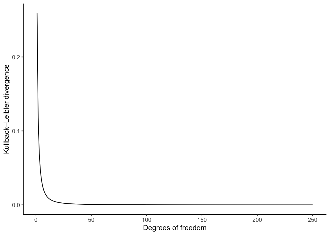

This plot looks at \(D_{KL}(P_{normal} \parallel P_t)\). Pretty quickly the KL-divergence plummets, leaving us with a pretty convincing approximation of the standard normal.

Mathematically

It’s important here that we’re approaching the standard normal, with \(\mu = 0\) and \(\sigma = 1\). The student’s t distribution doesn’t take any location or scale parameters, only degrees of freedom. The PDF for the standard normal is \[P_{normal}(x) = \frac{1}{\sqrt{2\pi}} e^{-\frac{x^2}{2}}\]

For student’s t, we have \[P_{t}(x, \nu) = \frac{\Gamma(\frac{\nu+1}{2})}{\sqrt{\nu\pi}\Gamma(\frac{\nu}{2})} \left( 1 + \frac{x^2}{\nu} \right)^{-\frac{\nu+1}{2}}\]

If you squint a little you might see a similarity, but its easy to miss. The most different looking part may be \(\frac{\Gamma \left ( \frac{\nu+1}{2} \right ) }{\sqrt{\nu\pi} \Gamma \left ( \frac{\nu}{2} \right )}\). We’ll call this part of the function the coefficient part. The coefficient part has two references to the Gamma function, but we dont need to worry about what that means today². Lets see how it looks under various degrees of freedom.

f <- function(nu) { gamma((nu+1)/ 2) / (sqrt(nu*pi) * gamma(nu/2)) }
df <- data.frame(dfs=1:250, coef=f(1:250))

ggplot(df, aes(x=dfs, y=coef)) + 
  geom_line() + 
  geom_hline(yintercept = 1/(sqrt(2*pi)), color='red') + 
  theme_classic() + ylab('Coefficient Part') + xlab('Degrees of freedom')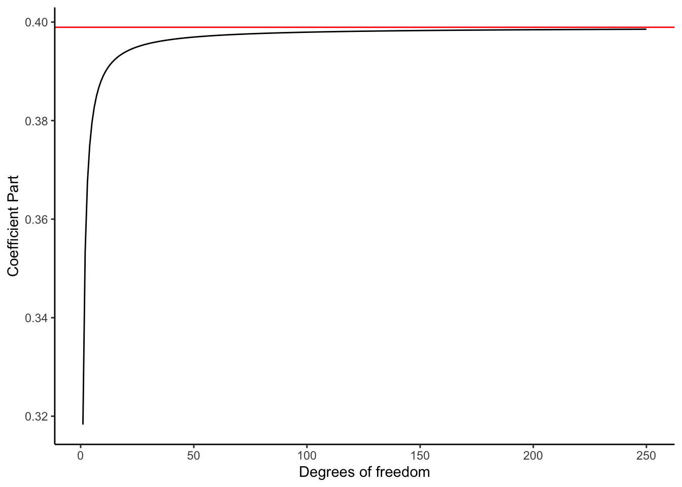

As \(nu\) increases, the coefficient part asymptotically approaches a number just below 0.4. And as you’ve probably guessed, \(1 / \sqrt{2\pi}\) is just under 0.4! As degrees of freedom go up, this part starts to look very much like the standard normal.

Now we have to consider the other part, \((1 + x^2 / \nu)^{-\frac{\nu+1}{2}}\). We’ll call this the main term, since it contains \(x\), the value we’re trying to get the probability density for. If we instead write the part as \(((1 + x^2 / \nu)^{\nu+1})^{-1/2}\), we can see something sort of familiar. One way of defining the exponential function is \(e^x = \lim_{n\rightarrow \infty} (1 + x^2/n )^n\). Now the t distribution has \(\nu+1\) in the exponent, so it won’t ever precisely meet \(e^x\), but it will get close.

Lets visualise the main term of both the t and standard normal distributions. Unlike the coefficient part, this is a function of \(x\), so we’ll animate the function over a range of degrees of freedom.

for (nu in 1:50) {
  f <- function(x) { (1 + (x^2/nu))^(-(nu+1)/2) }
  normf <- function(x) { exp(-(x^2/2)) }
  p <- ggplot(data.frame(x=c(-5,5)), aes(x)) + 
    stat_function(fun=normf, color='gray') + 
    stat_function(fun=f, color='blue') +
    theme_classic() + ylab("Result") + xlab('Value') + ggtitle(paste("df =", nu))
  print(p)
}

This animation looks a lot like our first animation. We’ve got a bell shape, and once again we see the the the t distribution rapidly approaching the standard normal. It’s easy to see why here: the coefficient parts of each distribution don’t change value with regard to the input value \(x\). These are just scaling factors that insure that these are actually probability distributions (i.e. that they integrate to 1). That scaling is what causes the dip around the center when you look at the whole distribution.

Of course, the \(t\) never becomes the normal. It asymptotically approaches the normal. But if you had an infinite sample size, you’d be looking at the standard normal.