library(tidyverse)

number_totals <- function(df) {
  ndf <- df %>% 
    distinct(player, year, number) %>% 
    group_by(number) %>% 
    summarise(n=n_distinct(player, year)) %>% 
    ungroup()
  
  # some numbers have never been used.
  missing_numbers <- setdiff(as.character(1:99), ndf$number)
  if (length(missing_numbers)) {
    missings <- data.frame(number=missing_numbers)
    missings$n <- 0
    
    ndf <- rbind(ndf, missings)
  }
  # function to numerically sort strings
  numsort <- function(v) { str_sort(v, numeric=T)}
  ndf %>% mutate(number=factor(number))  %>% mutate(number=fct_relevel(number, numsort))
}

plot_numbers <- function(df) {
  ticks <- c('0', '1', '10', '20', '30', '40', '50','60','70','80','90')
  df %>% 
    number_totals() %>%
    ggplot(aes(x=number, y=n)) + 
      geom_bar(stat='identity') + 
      scale_x_discrete(breaks=ticks) + 
      ylab("Player Seasons") + 
      xlab("Jersey Number") + 
      theme_classic()
}

Basketball

basketball-reference.com has NBA jersey numbers going back to the 1946-47 season (technically BAA jersey numbers in those years, since it wasn’t the NBA yet.)¹

nba <- read_csv("nba.csv")

## Parsed with column specification:
## cols(
##   player = col_character(),
##   year = col_double(),
##   number = col_character()
## )

plot_numbers(nba)

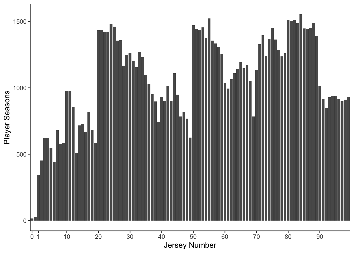
In the NBA we see a pretty chunky pattern. NBA players seem to prefer jerseys ending in digits 0-5. As it turns out while the NBA doesn’t have any rule requiring jersey numbers to be chosen this way, the NCAA does. Players want to keep their old numbers that they are comfortable with, so the NBA ends up reflecting that. The relative lack of numbers greater than 55 is a reflection of the same rule.

Football

pro-football-reference.com gives us player numbers as far back as 1947. So let’s take a look.

nfl <- read_csv("nfl.csv")

## Parsed with column specification:
## cols(
##   player = col_character(),
##   year = col_double(),
##   number = col_character()
## )

plot_numbers(nfl)

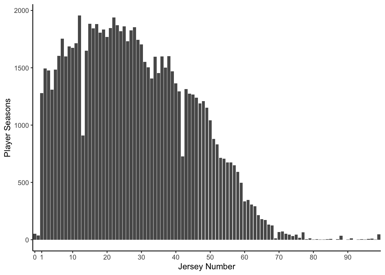
The NFL has the strongest rules about uniform numbers. Blocks of numbers are reserved for different positions, allowing the refs to know who is eligible to do what during a play. Thats why we see the pretty broad spread between 1 and 99. 0 and 00 are both rare though.

Baseball

baseball-reference.com gives us uniform numbers going back to 1923.

mlb <- read_csv('mlb.csv')

## Parsed with column specification:
## cols(
##   player = col_character(),
##   year = col_double(),
##   number = col_character()
## )

plot_numbers(mlb)

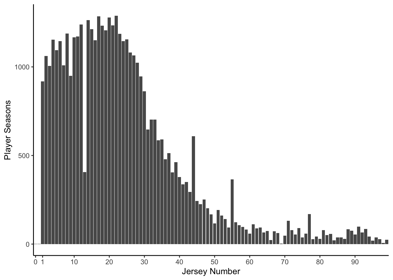
Baseball is a game of traditions. One of those is that players prefer lower numbers, leaving higher numbers for minor league players. There’s not a lot of players wearing unlucky #13 here. #47 was retired in the 1990s league-wide in honor of Jackie Robinson, explaining that dip.

Hockey

Lets look at hockey. hockey-reference.com has player numbers for the NHL going back to the 1950-1951 season.

nhl <- read_csv('nhl.csv')

## Parsed with column specification:
## cols(
##   player = col_character(),
##   year = col_double(),
##   number = col_character()
## )

plot_numbers(nhl)

NHL Players tend to prefer lower numbers. Number 1 is usually reserved for goalies, and the next few numbers for defensemen.² Unlucky #13 is usually not picked. NHL players do not use #0 or #00 generally.

Which fits best?

nba2 <- nba %>% 
  distinct(player, year, number) %>%
  group_by(number) %>% 
  summarise(n=n_distinct(player, year)) %>% 
  mutate(sport='NBA')

nfl2 <- nfl %>% 
  distinct(player, year, number) %>%
  group_by(number) %>% 
  summarise(n=n_distinct(player, year)) %>% 
  mutate(sport='NFL')

mlb2 <- mlb %>% 
  distinct(player, year, number) %>%
  group_by(number) %>% 
  summarise(n=n_distinct(player, year)) %>% 
  mutate(sport='MLB')

nhl2 <- nhl %>% 
  distinct(player, year, number) %>%
  group_by(number) %>% 
  summarise(n=n_distinct(player, year)) %>%
  mutate(sport='NHL')

numsort <- function(v) { str_sort(v, numeric=T)}
 
sports <- rbind(nba2, nfl2, mlb2, nhl2) %>% mutate(number=factor(number))  %>% mutate(number=fct_relevel(number, numsort))

number_counts <- sports %>% group_by(number) %>% summarise(n=sum(n)) %>% ungroup() %>% arrange(desc(n))

ticks <- c('0', '1', '10', '20', '30', '40', '50','60','70','80','90')
ggplot(sports, aes(x=number, y=n, fill=sport)) + geom_bar(stat='identity') + theme_classic() + scale_x_discrete(breaks=ticks) + xlab("Uniform Number") + ylab('Player-Seasons')

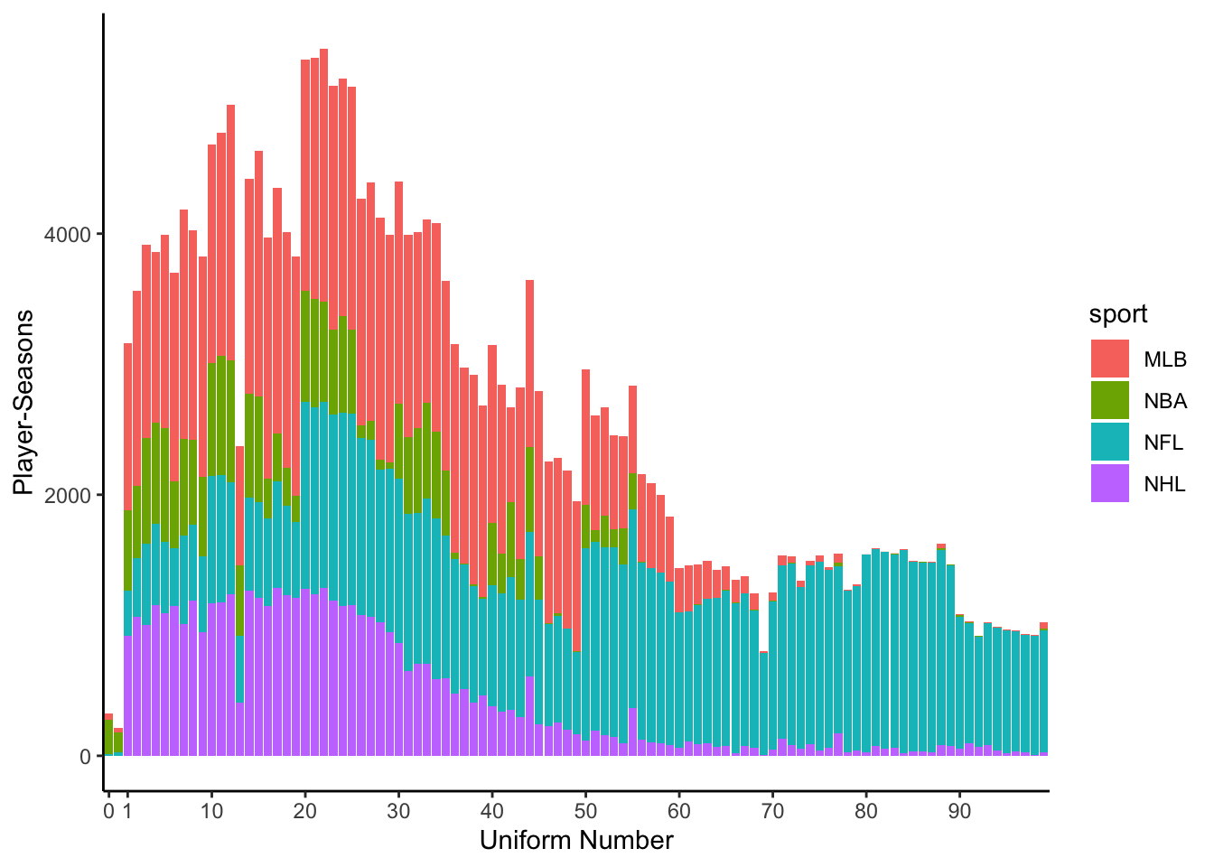
Ignoring league-size effects, the most common number is 22. Anything over 70 is just an NFL number. Any double-digit number where the ones digit is greater than 5 outs you as a non-basketball player. Combine that with the MLB and NHL preference for smaller jersey numbers, and the 20s are your best bet.