Why Do Random Forests Work?

When I was in seventh grade ‘life sciences’ class I was introduced to the concept of a dichotomous key. A dichotomous key is a tool for identifying organisms. It’s a flow chart that asks you question, and as you follow it, it helps you figure out what you’re looking at. For example: “does this animal have four legs” (yes), “does this animal have hair/fur?” (Yes), “does this animal have horns?” (No), “does this animal have hooves” (yes) might identify the animal you’re looking at as a “horse”.

A decision tree is basically a dichotomous key that you build from your data. It’s a flow chart of rules that you learn from your data to get a final prediction. A decision tree is basically the most naïve idea of what artificial intelligence is a bunch of nested if-else statements.

We don’t want to make these rules ourself though. We’d like our rules to be learned from the data. There are a couple different algorithms that differ on how they learn the rules, but in essence they do a similar thing. They take the data they’re learning from, and try to find the best way to split it: the best variable and cutoff value results in ‘pure’ outputs¹. The groups on each side of the split should be as homogenous as possible². Then repeat process for the data on each side.

A decision tree will do this forever: until it has perfectly learned from the training data. That’s usually not a great property: trees learned from your training data may not perform well in new data. This lack of generalizability is overfitting and it’s a problem for decision trees. As a result, the decision tree algorithms have a lot of hyperparameters you can tune in the learning process. Most of them have to do with when to stop learning, and that’s something you’ll have to figure out with cross-validation or a similar strategy.

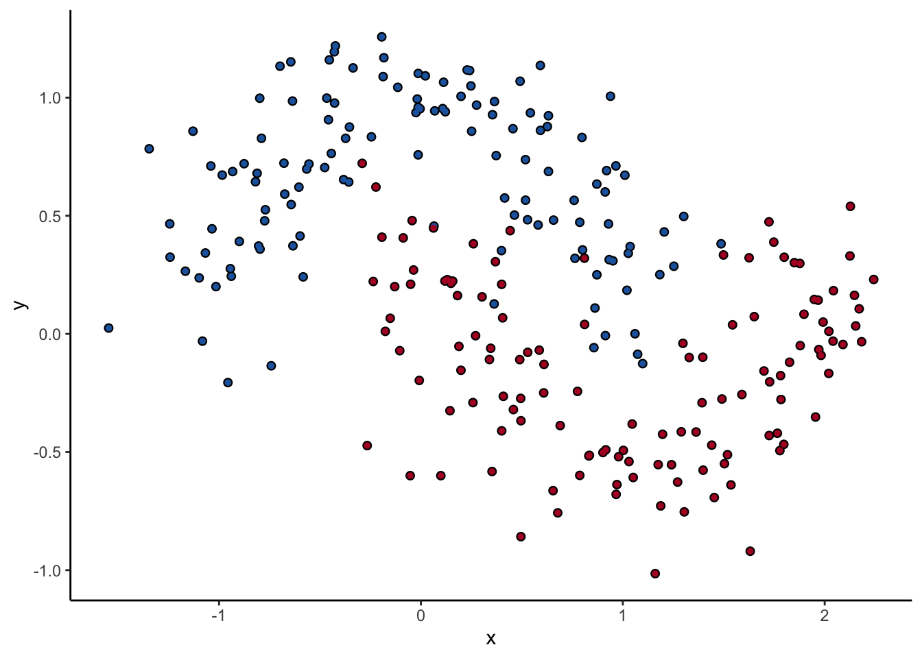
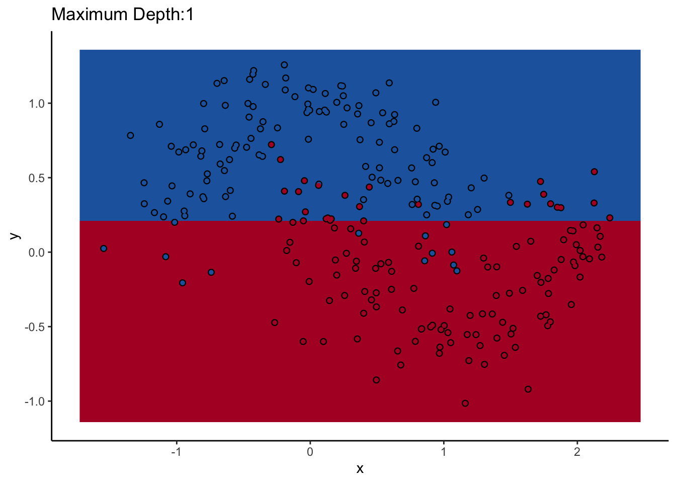
Let’s look at one of them. The scikit-learn DecisionTreeClassifer estimator has the hyperparameter max_depth, which controls how many splits you make before you stop learning. The dataset we’ll use for the rest of the post is two interlocking half-moons made with the make_moons function in scikit-learn. Obviously a linear classifier like logistic regression won’t work. A tree will probably work, but how well it performs remains to be seen.

How does max_depth affect performance? Let’s look at what it does as we increase it.

An individual decision tree is a finicky thing. There are certain decision boundaries they can have trouble learning without a large number of splits, and if you give them the room to learn them they’ll overfit. The random forest approach is an ensemble model: it uses many decision trees to compute an overall prediction that (usually) has better performance than any individual tree in the ensemble.

We’d like to use many trees to make the prediction, but if you give the tree algorithms the same input, you’ll get the same output for every tree in the forest. We need trees that vary meaningfully. The random forest is a bagging (short for bootstrap aggregation) ensemble. In this technique we sample (with replacement³) from our training dataset, and each tree looks at a different subsample from the dataset. The random forest goes a step further than an ordinary bagging model though. When considering splits, each tree only looks at a subset of the features as well. We’ve reduced both columns and rows.

The goal of this double subsetting is to have your trees be more independent of each other. Once you have independent trees, your forest takes each prediction and averages them all together to have an overall prediction. I don’t mean that as a simplification of some complicated math: you can add up all the predictions and divide by the total number of trees to make your final prediction. It’s that simple.

This double subsetting gives some other big advantages. The subsetting on rows means that you can test each tree’s performance on the datapoints it wasn’t trained on—the ‘out of bag’ data—which gives you another way to measure model performance (I’d still also use cross validation anyway). The subsetting on features lets you compare trees with and without an individual feature, which provides a measure of feature importance. Feature importance isn’t as enlightening as you might like (it doesn’t give you the effect of the predictor on performance for example), but in a world of black box machine learning models, feature importance really does add some interpretability to a model.

By using multiple trees, you also get a better idea of your predictions confidence⁴. In theory, there’s nothing stopping (in the sense that it’s not impossible) an individual tree from giving you a low confidence prediction. In practice though, decision trees try to find ‘pure’ leaf nodes: every point in the final node should be the same class. As a result, the individual trees are very confident of their predictions, even when they shouldn’t be. When you average multiple trees with different decision surfaces, you in effect ‘smooth’ out the boundaries between classes. Your class predictions will get farther away from 0 and 1, but that’s what you want near the boundary.

One big advantage of random forests over other models is the simplicity. It makes almost no assumptions about your data. And there’s minimal optimization involved. Finding the minimum of a function is often the root of overfitting in machine learning, and random forests doesn’t actually do any optimization⁵. The individual trees do when they make their splits, but even that isn’t necessary. There’s a variant of random forests called extremely randomized trees, where the individual trees that comprise the ensemble don’t even try to find good splits, they just pick a random cutoff between the minimum and maximum value of the feature.

Each tree in a random forest doesn’t know anything about what the other trees are doing. Because of that, the random forest is extremely parallelizable. It’s trivial to implement on multiple cores or CPUs to reduce training time. This is less true of boosted tree ensembles (like XGboost), in which the ensemble optimizes its performance by creating trees to address misclassifications by the previous tree in the model.

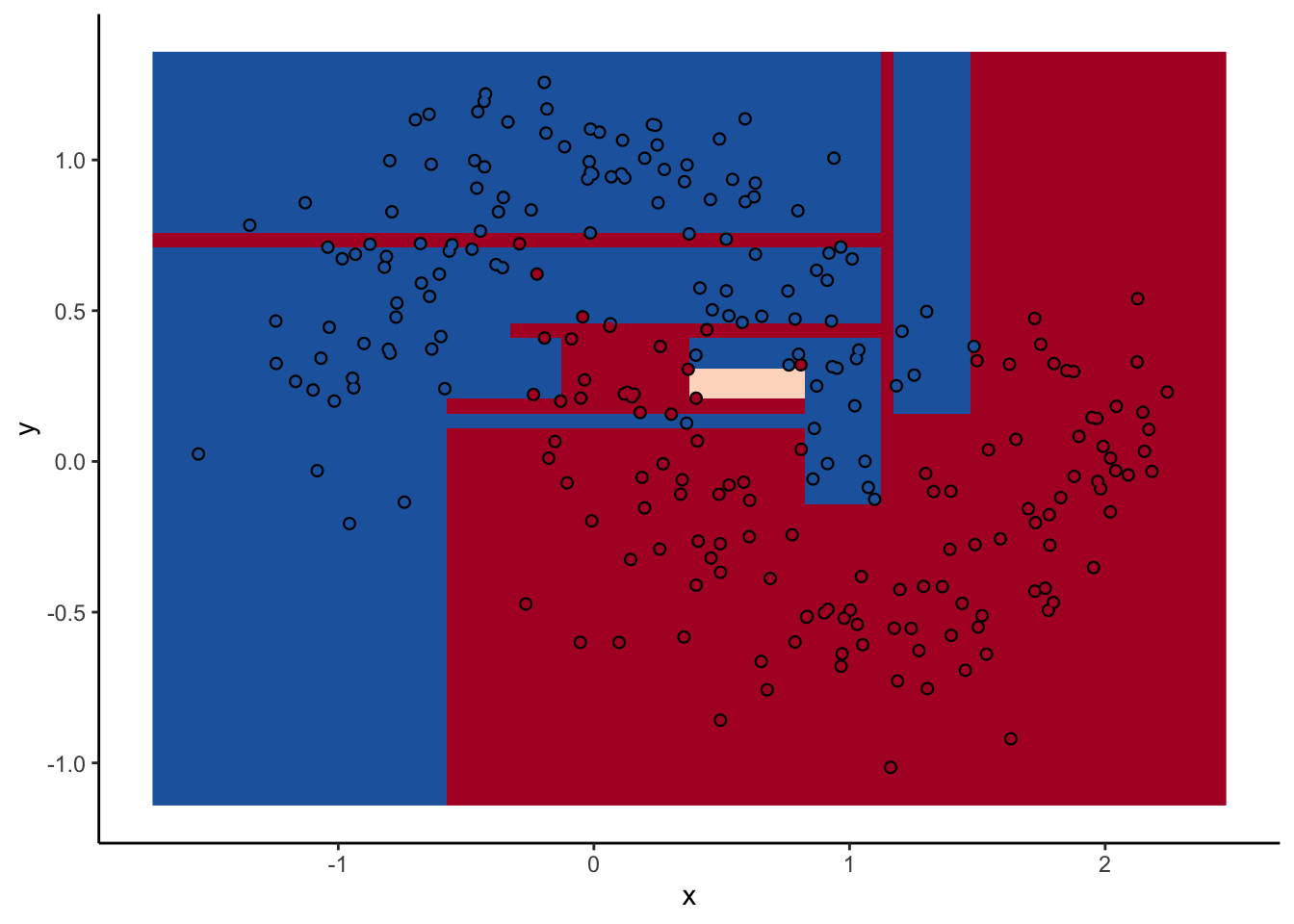
In a random forest, each individual tree can give some not-great performance⁶ without being altogether wrong. Look at this one:

With a two-dimensional toy example like we’re working with here, we can even look at every tree. This animation goes really fast, because I want to stress that the goal isn’t to diagnose how each tree is behaving at the decision boundary. The goal is to see where they agree.

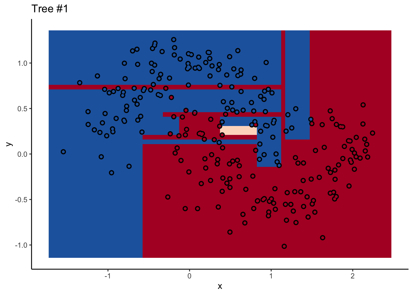
Each tree comes up with a so-so result. Not necessarily terrible (they mostly have the right idea), but making some odd decisions here and there that might burn you if you’re taking into production as the only estimator. What’s important is that they don’t all make the same mistake. Each tree makes its own unique mistakes. When we use a random forest, we average over all the trees, so these individual mistakes aren’t so prominent in the final output.

In the animation we can see that as we add more trees, the model refines its decision boundary more and more. The boundary isn’t a hard border now either. It transitions into a region of lower confidence as it moves between classes.

We can also see the artifacts of individual trees are still evident. The vertical and horizontal ‘streaks’⁷ but get washed out somewhat by the other trees that don’t make the same decision. Some areas without much data have low confidence, as the trees are focusing on other areas and it doesn’t matter how those regions are predicted since we can’t guage our accuracy there anyway.

The ‘wisdom of crowds’ aspect of random forest is what makes it such a great model. As a result of the averaging the random forests are very robust to noise and outliers. Performance will improve as you add trees to the forest, but you’ll run into diminishing returns after a few hundred trees. You can do some hyperparameter tuning to improve performance but the out of the box setting will get you a pretty good model⁸. It’s a baseline I include whenever I can.